Aggregation

An Aggregation (noun) is a set of specific calculations applied to data or previously calculated statistics. For example, an aggregation might calculate a single value, such as the average time (in seconds) it takes for RFQs to receive a price within a 10-second window.

Aggregation (verb) is the act of calculating stats from data. Aggregation can occur at the following places in Beeks Analytics:

1. Stack Probes in VMX-Capture
   A Statistics Collector (or stat collector) is a module in a stack probe that aggregates data to generate statistics from the observed traffic, which it then writes to a downstream component such as VMX-Analysis via a Generic Aggregator Input Event (GAIE) Connector.
   
   These are usually only the stats that require a lot of data, e.g., microburst detection. In a microburst example, a VMX-Capture Statistics Collector records the bandwidth measured in a 1 millisecond window, and records the mean, low, average and maximum value seen in each 10 second period. We generate microburst statistics in VMX-Capture as an efficiency measure, because passing large volumes of data to VMX-Analysis may result in the need for additional checking of timings to guarantee precision.
   
   When these stats are passed to VMX-Analysis for use in further aggregation, we refer to them as Pre-aggregated Stats. When these stats are passed to the Core Data Feed, we refer to them as stats.
   

2. VMX-Analysis
   Aggregation in VMX-Analysis performs calculations on Agent Event data and on Pre-aggregated Stats.
   

3. P3 Process
   The P3 process also generates Pre-aggregated Stats for further aggregation in VMX-Analysis. However, this pre-aggregation differs from the pre-aggregation in Stack Probes.
   
   P3 pre-aggregation is used when the volume of messages is exceptionally high and cannot be handled efficiently by Stack Probes alone. In this scenario, the message load is split between multiple Stack Probes, and these probe outputs are then split between multiple P3 processes. P3 can then rollup buckets of distribution to VMX-Analysis to get effective HDR distributions for high message volume calculations.

What are Aggregators?

Aggregators perform aggregation. One Aggregator can perform multiple aggregations.

In Beeks Analytics, Aggregators generate stats that are hierarchical, so that you can view top-level summaries and then more granular stats. We think of this hierarchy as a tree, with a root node, branch nodes, and leaf nodes.

A lot of the data you’ll see in VMX-Explorer dashboards is the output of one or more aggregations in an Aggregator.

Aggregation - a worked example

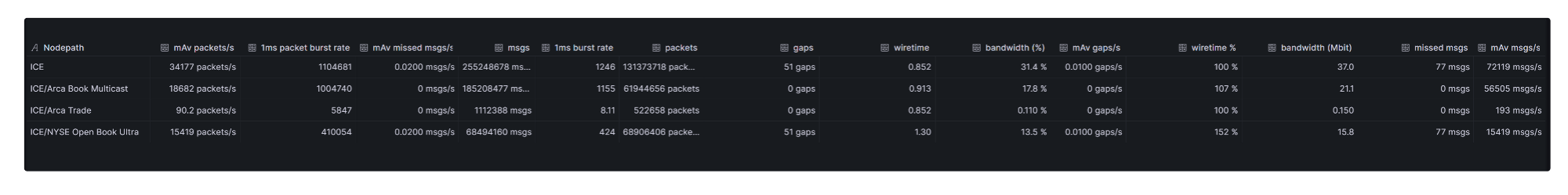
Let’s look at a simple example of one panel that displays the output from the aggregations in an Aggregator in a table.

In the example below, the nodepath column on the far-left includes ICE and ICE/Arca Trade. These are nodepaths that represent a branch node, i.e. summary stats for ICE, and a leaf node i.e., more granular stats for Arca Trade within ICE. Generally, an Aggregator offers top level summary data and multiple levels of breakdown by technical or business attributes.

We can see in the screenshot the familiar aggregator structure, standard for Beeks Analytics, which resembles a spreadsheet that represents a flattened tree structure, in which each cell is tracking a different stat.

Alternative worked example using CDF and a flat data model

If you are using CDF-T to output individual stats to a Time-series database, you can choose to retain the fixed hierarchical nodepath model or you can implement your own alternative data model.

If we take the earlier example market data aggregation, which uses a nodepath of vp/extgroup/switchport/feed/side/channel, we might see an aggregation like the following:

The ‘340’ and ‘2.68ms’ values might represent the latest values, but using the timeseries database functions you would be able to query previous values.

The above aggregation might have resulted from a stat update which published to the full nodepath:

This would be the traditional Beeks Analytics way of publishing the statistics update.

However, the above aggregation might also have resulted from a dynamic query-time reaggregation of the following data individual statistic update from CDF-T:

In the above case, the database table might look more like the following:

The columns for switchport and channel have been excluded from the example

The advantage of publishing the data in this second way is that you have the flexibility to group the data by, for example, “side”, giving you the mAv packets/s and mAv wiretime stats for all A and B sides e.g.,

This flexibility is not possible where statistics are published with a fixed nodepath.